2733. How the Universe Makes Gold

By Duncan Brown and Edo Berger, The Conversation, October 22, 2017

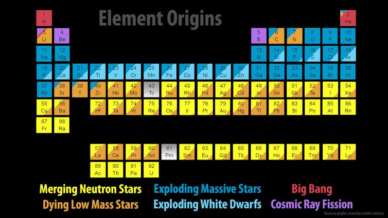
The electromagnetic radiation captured from GW170817 now confirms that elements heavier than iron are synthesized in the aftermath of neutron star collisions. Jennifer Johnson/SDSS, CC BY

For thousands of years, humans have searched for a way to turn matter into gold. Ancient alchemists considered this precious metal to be the highest form of matter. As human knowledge advanced, the mystical aspects of alchemy gave way to the sciences we know today. And yet, with all our advances in science and technology, the origin story of gold remained unknown. Until now.

Finally, scientists know how the universe makes gold. Using our most advanced telescopes and detectors, we’ve seen it created in the cosmic fire of the two colliding stars first detected by LIGO via the gravitational wave they emitted.

Origins of our elements

Scientists have been able to piece together where many of the elements of the periodic table come from. The Big Bang created hydrogen, the lightest and most abundant element. As stars shine, they fuse hydrogen into heavier elements like carbon and oxygen, the elements of life. In their dying years, stars create the common metals – aluminum and iron – and blast them out into space in different types of supernova explosions.

For decades, scientists have theorized that these stellar explosions also explained the origin of the heaviest and most rare elements, like gold. But they were missing a piece of the story. It hinges on the object left behind by the death of a massive star: a neutron star. Neutron stars pack one-and-a-half times the mass of the sun into a ball only 10 miles across. A teaspoon of material from their surface would weigh 10 million tons.

Many stars in the universe are in binary systems – two stars bound by gravity and orbiting around each other (think Luke’s home planet’s suns in “Star Wars”). A pair of massive stars might eventually end their lives as a pair of neutron stars. The neutron stars orbit each other for hundreds of millions of years. But Einstein says that their dance cannot last forever. Eventually, they must collide.

Massive collision, detected multiple ways

On the morning of August 17, 2017, a ripple in space passed through our planet. It was detected by the LIGO and Virgo gravitational wave detectors. This cosmic disturbance came from a pair of city-sized neutron stars colliding at one third the speed of light. The energy of this collision surpassed any atom-smashing laboratory on Earth.

Hearing about the collision, astronomers around the world, including us, jumped into action. Telescopes large and small scanned the patch of sky where the gravitational waves came from. Twelve hours later, three telescopes caught sight of a brand new star – called a kilonova – in a galaxy called NGC 4993, about 130 million light years from Earth.

Astronomers had captured the light from the cosmic fire of the colliding neutron stars. It was time to point the world’s biggest and best telescopes toward the new star to see the visible and infrared light from the collision’s aftermath. In Chile, the Gemini telescope swerved its large 26-foot mirror to the kilonova. NASA steered the Hubble to the same location.

Movie of the visible light from the kilonova fading away in the galaxy NGC 4993, 130 million light years away from Earth.

Just like the embers of an intense campfire grow cold and dim, the afterglow of this cosmic fire quickly faded away. Within days the visible light faded away, leaving behind a warm infrared glow, which eventually disappeared as well.

Observing the universe forging gold

But in this fading light was encoded the answer to the age-old question of how gold is made.

Shine sunlight through a prism and you will see our sun’s spectrum – the colors of the rainbow spread from short wavelength blue light to long wavelength red light. This spectrum contains the fingerprints of the elements bound up and forged in the sun. Each element is marked by a unique fingerprint of lines in the spectrum, reflecting the different atomic structure.

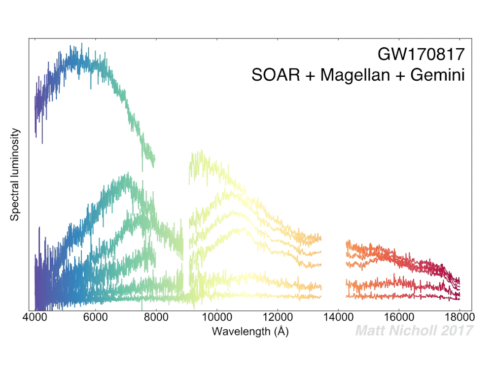
The spectrum of the kilonova contained the fingerprints of the heaviest elements in the universe. Its light carried the telltale signature of the neutron-star material decaying into platinum, gold and other so-called “r-process” elements.

Visible and infrared spectrum of the kilonova. The broad peaks and valleys in the spectrum are the fingerprints of heavy element creation. Matt Nicholl, CC BY

For the first time, humans had seen alchemy in action, the universe turning matter into gold. And not just a small amount: This one collision created at least 10 Earths’ worth of gold. You might be wearing some gold or platinum jewelry right now. Take a look at it. That metal was created in the atomic fire of a neutron star collision in our own galaxy billions of years ago – a collision just like the one seen on August 17.

And what of the gold produced in this collision? It will be blown out into the cosmos and mixed with dust and gas from its host galaxy. Perhaps one day it will form part of a new planet whose inhabitants will embark on a millennia-long quest to understand its origin.

2732. Fish Can Get Depressed

By Heather Murphy, The New York Times, October 12, 2017

Can a fish be depressed? This question has been floating around my head ever since I spent a night in a hotel across from an excruciatingly sad-looking Siamese fighting fish. His name was Bruce Lee, according to a sign beneath his little bowl.

There we were trying to enjoy a complimentary bloody mary on the last day of our honeymoon and there was Bruce Lee, totally still, his lower fin grazing the clear faux rocks on the bottom of his home. When he did finally move, just slightly, I got the sense that he would prefer to be dead.

The pleasant woman at the front desk assured me that he was well taken care of. Was I simply anthropomorphizing Bruce Lee, incorrectly assuming his lethargy was a sign of mental distress?

When I sought answers from scientists, I assumed that they would find the question preposterous. But they did not. Not at all.

It turns out that not only can our gilled friends become depressed, but some scientists consider fish to be a promising animal model for developing anti-depressants. New research, I would learn, has been radically shifting the way that scientists think about fish cognition, building a case that pet and owner are not nearly as different as many assume.

“The neurochemistry is so similar that it’s scary,” said Julian Pittman, a professor at the Department of Biological and Environmental Sciences at Troy University in Alabama, where he is working to develop new medications to treat depression, with the help of tiny zebrafish. We tend to think of them as simple organisms, “but there is a lot we don’t give fish credit for.”

Dr. Pittman likes working with fish, in part, because they are so obvious about their depression. He can reliably test the effectiveness of antidepressants with something called the “novel tank test.” A zebrafish gets dropped in a new tank. If after five minutes it is hanging out in the lower half, it’s depressed. If it’s swimming up top — its usual inclination when exploring a new environment — then it’s not.

The severity of the depression, he says, can be measured by quantity of time at the top vs. the bottom all of which seemed to confirm my suspicions about Bruce Lee.

All of this, of course, may sound fishy to any of the one in six people who has experienced clinical depression. How could a striped minnow relate to what you’ve been through? Is “depression” the right word?

While scientists have used animals, like mice, to study emotional problems for decades, the relevance of those models to human experience is sketchy at best.

There’s the obvious issue that “We cannot ask animals how they feel,” says Dr. Diego A. Pizzagalli, the director of the Center For Depression, Anxiety and Stress Research at Harvard Medical School. Though researchers may find parallels in serotonin and dopamine fluctuations, neither fish nor rat can “capture the entire spectrum of depression as we know it,” says Dr. Pizzagalli.

There is a heated debate in the fish research community about whether anxious or depressed is a more appropriate term.

But what has convinced Dr. Pittman, and others, over the past ten years is watching the way the zebrafish lose interest in just about everything: food, toys, exploration — just like clinically depressed people.

“You can tell,” said Culum Brown, a behavioral biologist at Macquarie University in Sydney who has published more than 100 papers on fish cognition. “Depressed people are withdrawn. The same is true of fish.”

The trigger for most domestic fish depression is likely lack of stimulation, said Victoria Braithwaite, a professor of fisheries and biology at Penn State University, who studies fish intelligence and fish preferences.

Study after study shows how fish are defying aquatic stereotypes: some fish use tools, others can recognize individual faces.

“One of the things we’re finding that fish are naturally curious and seek novel things out,” said Dr. Braithwaite. In other words, your goldfish is probably bored. To help ward off depression, she urges introducing new objects to the tank or switching up the location of items.

Dr. Brown agrees, pointing to an experiment he conducted, that showed that if you leave a fish in an enriched, physically complex environment — meaning lot of plants to nibble on and cages to swim through — it decreases stress and increases brain growth.

The problem with small tanks is not just the lack of space for exploration, said Dr. Brown, but also the water quality tends to be unstable and there may not be sufficient oxygen.

“A goldfish bowl for example is the worst possible situation,” he said.

If you own fish, you might want to consider where Dr. Brown keeps his: an extensively-landscaped six-foot tank. He recommends a “two foot tank with lots of plants and stuff” for your average betta.

The last time a guest posted Bruce Lee to Instagram he was looking good and lively. Perhaps that new green leaf in his bowl had provided the enrichment he craved.

But then, my heart sank. The internet produced photos of other Bruce Lees from the same hotel in several colors — red, blue and purplish. I wondered whether the monotony would eventually drive this replacement Bruce, to hover, immobile, near his transparent rocks.

2731. Wild and Captive Chimpanzees Share Personality Traits With Humans

By Karen Weintraub, The New York Times, October 24, 2017

In the late 1950s and early 1960s, Jane Goodall started attributing personalities to the chimpanzees she followed in Gombe National Park in what is now Tanzania. In her descriptions, some were more playful or aggressive, affectionate or nurturing.

Many scientists at the time were horrified, she recalled. Considered an amateur — she didn’t yet have her Ph.D. — they contended she was inventing personality traits for animals.

Dr. Goodall, now 83, said in a phone interview on Monday from her home in England that scientists thought “I was guilty of the worst kind of anthropomorphism.”

But time has borne out her insights. Chimpanzees in the wild have personalities similar to those in captivity, and both strongly overlap with traits that are familiar in humans, a new study published in Scientific Data confirms.

The new examination of chimpanzees at Gombe updates personality research conducted on 24 animals in 1973 to include more than 100 additional chimps that were evaluated a few years ago. The animals were individually assessed by graduate students in the earlier study, and in the latest by Tanzanian field assistants, on personality traits like agreeableness, extroversion, depression, aggression and self-control.

Researchers used different questionnaires to assess the chimps’ traits in the two studies, but most of the personality types were consistent across the two studies.

These traits seen among wild chimps matched ones seen among captive animals, the study found, and are similar to those described in people.

Dr. Goodall, who is promoting a new documentary, “Jane,” about those early days of her research, said she’s not surprised. She knew from childhood experiences with guinea pigs, tortoises and her favorite dog, Rusty, that animals have personalities that are quite familiar.

“I honestly don’t think you can be close to any animals and not realize their very vivid personalities,” she said.

Clive Wynne, a professor and director of the Canine Science Collaboratory at Arizona State University in Tempe, who was not involved in the research, said the new study offered a “really rich picture” of the overlap among species.

“It’s backing up and reinforcing a number of things that we assume about animal personality that are seldom established with this degree of security in substantial wild-living populations,” said Dr. Wynne, who concurs that dogs, his area of specialty, also have similar personality traits.

Robert Latzman, an associate professor at Georgia State University, who was not involved in the study, said his research with chimpanzees in zoos has always left open the question of whether animals in the wild are somehow different.

“What’s exciting about these data is there’s some suggestion that wild apes look very similar to what we would expect in terms of basic dispositional traits and continuity of those traits — and I don’t mean just to captive chimpanzees, but to humans,” he said. “The work in the wild underscores how similar these animals truly are to humans.”

Alexander Weiss, who led the new study, said he was particularly interested in examining the personality traits of animals in the wild. His findings were in line with previous research he’s done on chimpanzees in captivity.

“The fact that we’re showing this consistency in the wild is nice, because it allows us to draw more general conclusions,” said Dr. Weiss, a senior lecturer at the University of Edinburgh. “It’s not just being in a zoo that’s causing these individual traits to be stable.”

The study’s underlying data will be made publicly available so other scientists can use them in their own research, he said.

Although most of the animals tested in 1973 had died by the time the recent analysis was conducted, the study also concluded that an animal’s personality traits were generally consistent over time.

Dr. Goodall said that fits what she’s seen, too. She only visits Gombe twice a year now, and only two animals are still alive from the days when she knew them as individuals. One, a mother of twins named Gremlin, has changed a bit, Dr. Goodall said.

“I think the main difference in her personality is she’s become more confident as she gets older, just like people do,” she said.

Dr. Goodall added that she’s pleased that researchers are still finding so much of interest at Gombe, and tapping into the expertise of Tanzanian field workers.

And, of course, she’s happy that the academic perspective has shifted from the time when she was told only humans had personalities, minds and emotions.

“Today you can get your Ph.D. studying animal personality. I think we’ve come around full-cycle,” she said. “It absolutely vindicates all that I’ve ever believed.”

2730. Insectageddon: Farming Is More Catastrophic Than Climate Breakdown

By George Monbiot, The Guardian, October 20, 2017

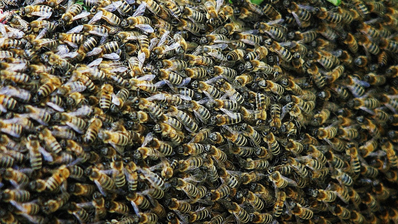
Honeybee colony collapse disorder is caused by multiple factors, including neonicotinoids. 

Which of these would you name as the world’s most pressing environmental issue? Climate breakdown, air pollution, water loss, plastic waste or urban expansion? My answer is none of the above. Almost incredibly, I believe that climate breakdown takes third place, behind two issues that receive only a fraction of the attention.

This is not to downgrade the danger presented by global heating – on the contrary, it presents an existential threat. It is simply that I have come to realise that two other issues have such huge and immediate impacts that they push even this great predicament into third place.

One is industrial fishing, which, all over the blue planet, is now causing systemic ecological collapse. The other is the erasure of non-human life from the land by farming.

And perhaps not only non-human life. According to the UN Food and Agriculture Organisation, at current rates of soil loss, driven largely by poor farming practice, we have just 60 years of harvests left. And this is before the Global Land Outlook report, published in September, found that productivity is already declining on 20% of the world’s cropland.

The impact on wildlife of changes in farming practice (and the expansion of the farmed area) is so rapid and severe that it is hard to get your head round the scale of what is happening. A study published this week in the journal Plos One reveals that flying insects surveyed on nature reserves in Germany have declined by 76% in 27 years. The most likely cause of this Insectageddon is that the land surrounding those reserves has become hostile to them: the volume of pesticides and the destruction of habitat have turned farmland into a wildlife desert.

It is remarkable that we need to rely on a study in Germany to see what is likely to have been happening worldwide: long-term surveys of this kind simply do not exist elsewhere. This failure reflects distorted priorities in the funding of science. There is no end of grants for research on how to kill insects, but hardly any money for discovering what the impacts of this killing might be. Instead, the work has been left – as in the German case – to recordings by amateur naturalists.

But anyone of my generation (ie in the second bloom of youth) can see and feel the change. We remember the “moth snowstorm” that filled the headlight beams of our parents’ cars on summer nights (memorialised in Michael McCarthy’s lovely book of that name). Every year I collected dozens of species of caterpillars and watched them grow and pupate and hatch. This year I tried to find some caterpillars for my children to raise. I spent the whole summer looking and, aside from the cabbage whites on our broccoli plants, found nothing in the wild but one garden tiger larva. Yes, one caterpillar in one year. I could scarcely believe what I was seeing – or rather, not seeing.

Insects, of course, are critical to the survival of the rest of the living world. Knowing what we now know, there is nothing surprising about the calamitous decline of insect-eating birds. Those flying insects – not just bees and hoverflies but species of many different families – are the pollinators without which a vast tract of the plant kingdom, both wild and cultivated, cannot survive. The wonders of the living planet are vanishing before our eyes.

Well, I hear you say, we have to feed the world. Yes, but not this way. As a UN report published in March explained, the notion that pesticide use is essential for feeding a growing population is a myth. A recent study in Nature Plants reveals that most farms would increase production if they cut their use of pesticides. A study in the journal Arthropod-Plant Interactions shows that the more neonicotinoid pesticides were used to treat rapeseed crops, the more their yield declines. Why? Because the pesticides harm or kill the pollinators on which the crop depends.

Farmers and governments have been comprehensively conned by the global pesticide industry. It has ensured its products should not be properly regulated or even, in real-world conditions, properly assessed. A massive media onslaught by this industry has bamboozled us all about its utility and its impacts on the health of both human beings and the natural world.

The profits of these companies depend on ecocide. Do we allow them to hold the world to ransom, or do we acknowledge that the survival of the living world is more important than returns to their shareholders? At the moment, shareholder value comes first. And it will count for nothing when we have lost the living systems on which our survival depends.

To save ourselves and the rest of the living world, here’s what we need to do:

1 We need a global treaty to regulate pesticides, and put the manufacturers back in their box.

2 We need environmental impact assessments for the farming and fishing industries. It is amazing that, while these sectors present the greatest threats to the living world, they are, uniquely in many nations, not subject to such oversight.

3 We need firm rules based on the outcomes of these assessments, obliging those who use the land to protect and restore the ecosystems on which we all depend.

4 We need to reduce the amount of land used by farming, while sustaining the production of food. The most obvious way is greatly to reduce our use of livestock: many of the crops we grow and all of the grazing land we use are deployed to feed them. One study in Britain suggests that, if we stopped using animal products, everyone in Britain could be fed on just 3m of our 18.5m hectares of current farmland (or on 7m hectares if all our farming were organic). This would allow us to create huge wildlife and soil refuges: an investment against a terrifying future.

5 We should stop using land that should be growing food for people to grow maize for biogas and fuel for cars.

Then, at least, nature and people would have some respite from the global onslaught. And, I hope, a chance of getting through the century.

2729. More Than 75 Percent Decline Over 27 Years in Total Flying Insect Biomass in Protected Areas

By Caspar A. Hallmann, Martin Sorg, Eelke Jongejans, Henk Siepel, Nick Hofland,Heinz Schwan,Werner Stenmans,Andreas Müller,Hubert Sumser,Thomas Hörren,Dave Goulson,Hans de Kroon, PLOS, October 18, 2017

Photo: Getty

Abstract

Global declines in insects have sparked wide interest among scientists, politicians, and the general public. Loss of insect diversity and abundance is expected to provoke cascading effects on food webs and to jeopardize ecosystem services. Our understanding of the extent and underlying causes of this decline is based on the abundance of single species or taxonomic groups only, rather than changes in insect biomass which is more relevant for ecological functioning. Here, we used a standardized protocol to measure total insect biomass using Malaise traps, deployed over 27 years in 63 nature protection areas in Germany (96 unique location-year combinations) to infer on the status and trend of local entomofauna. Our analysis estimates a seasonal decline of 76%, and mid-summer decline of 82% in flying insect biomass over the 27 years of study. We show that this decline is apparent regardless of habitat type, while changes in weather, land use, and habitat characteristics cannot explain this overall decline. This yet unrecognized loss of insect biomass must be taken into account in evaluating declines in abundance of species depending on insects as a food source, and ecosystem functioning in the European landscape.

Figures

   

Citation: Hallmann CA, Sorg M, Jongejans E, Siepel H, Hofland N, Schwan H, et al. (2017) More than 75 percent decline over 27 years in total flying insect biomass in protected areas. PLoS ONE12(10): e0185809. https://doi.org/10.1371/journal.pone.0185809

Editor: Eric Gordon Lamb, University of Saskatchewan, CANADA

Received: July 28, 2017; Accepted: September 19, 2017; Published: October 18, 2017

Copyright: © 2017 Hallmann et al. This is an open access article distributed under the terms of the Creative Commons Attribution License, which permits unrestricted use, distribution, and reproduction in any medium, provided the original author and source are credited.

Data Availability: All relevant data are within the paper and its Supporting Information files.

Funding: CH and EJ were supported by the Netherlands Organization for Scientific Research (NWO grants 840.11.001 and 841.11.007), and NH by the Triodos Foundation. The investigations of the Entomological Society Krefeld and its members are spread over numerous individual projects at different locations and in different years. Grants and permits that have made this work possible are listed below: Bezirksregierungen Düsseldorf & Köln, BfN - Bundesamt für Naturschutz, Land Nordrhein-Westfalen - Europäische Gemeinschaft ELER, Landesamt für Agrarordnung Nordrhein-Westfalen, Landesamt für Natur, Umwelt und Verbraucherschutz Nordrhein-Westfalen, Landesamt für Umwelt Brandenburg, Landesamt für Umwelt Rheinland-Pfalz, LVR - Landschaftsverband Rheinland, Naturschutzbund Deutschland, Nordrhein-Westfalen Stiftung, RBN Bergischer Naturschutzverein, RVR - Regionalverband Ruhr, SGD Nord Rheinland-Pfalz, Universitäten Bonn, Duisburg-Essen & Köln, Untere Landschaftsbehörden: Kreis Düren, Kreis Heinsberg, Kreis Kleve, Kreis Viersen, Kreis Wesel & AGLW, Stadt Düsseldorf, Stadt Köln, Stadt Krefeld, Rheinisch Bergischer Kreis, Rhein Kreis Neuss & Rhein-Sieg-Kreis. Members of the Entomological Society Krefeld and cooperating botanists and entomologists that were involved in the empirical investigations are greatly acknowledged: U.W. Abts, F. Bahr, A. Bäumler, D. & H. Beutler, P. Birnbrich, U. Bosch, J. Buchner, F. Cassese, K. Cölln, A.W. Ebmer, R. Eckelboom, B. Franzen, M. Grigo, J. Günneberg, J. Gusenleitner, K. Hamacher, F. Hartfeld, M. Hellenthal, J. Hembach, A. Hemmersbach, W. Hock, V. Huisman-Fiegen, J. Illmer, E. Jansen, U. Jäckel, F. Koch, M. Kreuels, P. Leideritz, I. Loksa, F. B. Ludescher, F. J. Mehring, G. Milbert, N. Mohr, P. Randazzo, K. Reissmann, S. Risch, B. Robert, J. de Rond, U. Sandmann, S. Scharf, P. Scherz, J. Schiffer, C. Schmidt, O. & W. Schmitz, B. P. & W. Schnell, J. L. Schönfeld, E. Schraetz, M. Schwarz, R. Seliger, H. W. Siebeneicher, F. & H. Sonnenburg W. J. S. & P. Sorg, A. Ssymank, H. Sticht, M. Weithmann, W. Wichard and H. Wolf.

Competing interests: The authors have declared that no competing interests exist.

Introduction

Loss of insects is certain to have adverse effects on ecosystem functioning, as insects play a central role in a variety of processes, including pollination [1, 2], herbivory and detrivory [3, 4], nutrient cycling [4] and providing a food source for higher trophic levels such as birds, mammals and amphibians. For example, 80% of wild plants are estimated to depend on insects for pollination [2], while 60% of birds rely on insects as a food source [5]. The ecosystem services provided by wild insects have been estimated at $57 billion annually in the USA [6]. Clearly, preserving insect abundance and diversity should constitute a prime conservation priority.

Current data suggest an overall pattern of decline in insect diversity and abundance. For example, populations of European grassland butterflies are estimated to have declined by 50% in abundance between 1990 and 2011 [7]. Data for other well-studied taxa such as bees [8–14] and moths [15–18] suggest the same trend. Climate change, habitat loss and fragmentation, and deterioration of habitat quality have been proposed as some of the prime suspects responsible for the decline [9–11, 13, 18–22]. However, the number of studies on insect trends with sufficient replication and spatial coverage are limited [10, 23–25] and restricted to certain well-studied taxa. Declines of individual species or taxa (e.g. [7, 26]) may not reflect the general state of local entomofauna [27]. The total insect biomass would then be a better metric for the status of insects as a group and its contribution to ecosystem functioning, but very few studies have monitored insect biomass over an extensive period of time [28]. Hence, to what extent total insect biomass has declined, and the relative contribution of each proposed factor to the decline, remain unresolved yet highly relevant questions for ecosystem ecology and conservation.

Here, we investigate total aerial insect biomass between 1989 and 2016 across 96 unique location-year combinations in Germany, representative of Western European low-altitude nature protection areas embedded in a human-dominated landscape (S1 Fig). In all years we sampled insects throughout the season (March through October), based on a standardized sampling scheme using Malaise traps. We investigated rate of decline in insect biomass, and examined how factors such as weather, habitat and land use variables influenced the declines. Knowledge on the state of insect biomass, and it’s direction over time, are of broad importance to ecology and conservation, but historical data on insect biomass have been lacking. Our study makes a first step into filling this gap, and provides information that is vital for the assessment of biodiversity conservation and ecosystem health in agricultural landscapes.

Materials and methods

Data

Biomass data.

Biomass data were collected and archived using a standardized protocol across 63 unique locations between 1989 and 2016 (resulting in 96 unique location-year combinations) by the Entomological Society Krefeld. The standardized protocol of collection has been originally designed with the idea of integrating quantitative aspects of insects in the status assessment of the protected areas, and to construct a long-term archive in order to preserve (identified and not-identified) specimens of local diversity for future studies. In the present study, we consider the total biomass of flying insects to assess the state of local entomofauna as a group.

All trap locations were situated in protected areas, but with varying protection status: 37 locations are within Natura2000 sites, seven locations within designated Nature reserves, nine locations within Protected Landscape Areas (with funded conservation measures), six locations within Water Protection Zones, and four locations of protected habitat managed by Regional Associations. For all location permits have been obtained by the relevant authorities, as listed in the S1 Appendix. In our data, traps located in nutrient-poor heathlands, sandy grasslands, and dune habitats provide lower quantities of biomass as compared to nutrient nutrient-rich grasslands, margins and wastelands. As we were interested in whether the declines interact with local productivity, traps locations were pooled into 3 distinct habitat clusters, namely: nutrient-poor heathlands, sandy grassland, and dunes (habitat cluster 1, n = 19 locations, Fig 1A), nutrient-rich grasslands, margins and wasteland (habitat cluster 2, n = 41 locations, Fig 1B) and a third habitat cluster that included pioneer and shrub communities (n = 3 locations).

Download:

• PPT
  PowerPoint slide
• PNG
  larger image
• TIFF
  original image

Fig 1. Examples of operating malaise traps in protected areas in western Germany, in habitat cluster 1 (A) and cluster 2 (B) (see Materials and methods).

https://doi.org/10.1371/journal.pone.0185809.g001

Most locations (59%, n = 37) were sampled in only one year, 20 locations in two years, five locations in three years, and one in four years, yielding in total 96 unique location-year combinations of measurements of seasonal total flying insect biomass. Our data do not represent longitudinal records at single sites, suitable to derive location specific trends (e.g. [28]). Prolonged trapping across years is in the present context (protected areas) deemed undesirable, as the sampling process itself can negatively impact local insect stocks. However, the data do permit an analysis at a higher spatial level, i.e. by treating seasonal insect biomass profiles as random samples of the state of entomofauna in protected areas in western Germany.

Malaise traps were deployed through the spring, summer and early autumn. They operated continuously (day and night), and catches were emptied at regular intervals, on average every 11.2 days (sd = 6.3). We collected in total 1503 trap samples, with an average of 16 (4–35) successive catches per location-year combination (Table 1). Between 1989 and 2016, a total of 53.54kg of invertebrates have been collected and stored, over a total trap exposure period of 16908 days, within an average of 176 exposure days per location-year combination. Malaise traps are known to collect a much wider diversity of insect species (e.g. [29–31]) as compared to suction traps (e.g. [28]) and are therefore considered superior as a method of collecting flying insects. On the basis of partial assessments, we can assume that the total number of insects included in 53.54 kg biomass represents millions of individuals.

Download:

• PPT
  PowerPoint slide
• PNG
  larger image
• TIFF
  original image

Table 1. Overview of malaise-trap samples sizes.

For each year, the number of locations sampled, the number of location re-sampled, total number of samples, as well as mean and standard deviation of exposure time at the trap locations (in days) are presented.

https://doi.org/10.1371/journal.pone.0185809.t001

The sampling was standardized in terms of trap construction, size and design (identical parts), colors, type of netting and ground sealing, trap orientation in the field as well as slope at the trap location. Hence none of the traps differed in any of these field aspects. Our trap model was similar to the bi-colored malaise trap model by Henry Townes [32, 33]. The traps, collecting design, and accompanying methods of biomass measurement as designed and applied by the Entomological Society Krefeld are described elsewhere [34–36] and in S2 Appendix.

Trap catches were stored in 80% ethanol solution, prior to weighing, and total insect biomass of each catch (bottle) was obtained based on a standardized measurement protocol by first subtracting fluid content. In order to optimally preserve samples for future species determination, the insects were weighed in an alcohol-wet state. First, the alcohol concentration in the vessels was stabilized to 80%, while this concentration was controlled with an areometer over a period of at least two days. In order to obtain biomass per sample with sufficient accuracy and comparability, the measuring process was fixed using a standardized protocol [34]. For this purpose the insects of a sample were poured onto a stainless steel sieve (10cm diameter) of 0.8 mm mesh width. This sieve is placed slightly obliquely (30 degrees) over a glass vessel. The skew position accelerates the first runoff of alcohol and thus the whole measuring procedure. The drop sequence is observed with a stopwatch. When the time between two drops has reached 10 seconds for the first time, the weighing process is performed with a laboratory scale. For the determination of the biomass, precision scales and analytical scales from Mettler company were used with an accuracy of at least 0.1g and controlled with calibrated test weights at the beginning of a new weighing series. In a series of 84 weightings of four different samples repeating this measurement procedure, an average deviation from the mean value of the measurement results of 0.4 percent was observed (unpublished results).

Weather data.

Climate change is a well-known factor responsible for insect declines [15, 18, 21, 37]. To test if weather variation could explain the observed decline, we included mean daily temperature, precipitation and wind speed in our analysis, integrating data from 169 weather stations [38] located within 100km to the trap locations. We examined temporal trends in each weather variable over the course of the study period to assess changes in climatic conditions, as a plausible explanation for insect decline. Estimates of each weather variable at the trap locations were obtained by interpolation of each variable from the 169 climate stations.

We initially considered mean daily air temperature, precipitation, cloud cover, relative air moisture content, wind speed, and sunshine duration. However, only temperature, precipitation and wind speed were retained for analysis, as the other variables were significantly correlated with the selected variables [R(temperature, cover) = −43.2%, R(temperature, sunshine) = 53.4%, R(precipitation, moisture) = −47.3%] and because we wanted to keep the number of covariates as low as possible. Additionally, we calculated the number of frost days and the sum of precipitation in the months November- February preceding a sampling season. We used spatio-temporal geostatistical models [39, 40] to predict daily values for each weather variable to each trap location. Amongst other methods, the geostatistical approach is considered a superior interpolation method in order to derive weather variables to trap locations [41]. Uncertainty in interpolated variables such as wind speed is usually associated with altitude differences. However, as our trap locations are all situated in lowland areas with little altitude variation, we do not expect a large error in our interpolations at trap locations.

We decomposed the daily values of each weather variable into a long-term average trend (between years), a mean seasonal trend, and a yearly seasonal anomaly component (S2 Fig), modeled using regression splines [42] while controlling for altitude of weather stations. The remaining residual daily values of each station were further modeled using a spatio-temporal covariance structure. For example, temperature T, on given day t, of a given year k at a given trap location s is modeled as:(1)where fk(k) is the long-term trend over the years (a thin plate regression spline), ft(t) the mean seasonal trend within years (a penalized cyclic cubic regression spline), r(k, t) the mean residual seasonal component, which measures annual anomaly in mean daily values across selected stations, and a is the linear coefficient for the altitude h effect. The spatio-temporal covariance structure Cs, t, fitted independently to the residuals of each weather variable model, allowed us to deal with lack of independence between daily weather data within and between stations, as well as to interpolate to trap locations using kriging. Altitude of trap locations was extracted from a digital elevation models at 90m resolution [43].

Land use data.

Land use variables (and changes therein) were derived from aerial photographs [44] taken within two distinct time periods (between 1989–1994, and between 2012–2015), and allowed us to characterize land use composition at surroundings of the traps, as well as changes over time. We distinguished cover of forests, agricultural areas, natural grassland, and surface water. For each trap location, aerial photographs were manually processed, polygons extracted and categorized, and their surface area calculated with a radius of 200 meter. Preliminary analysis of the relationship between log biomass and landuse variables, on a subset of the trap locations, indicated that land use elements at 200m radius better predicted insect biomass than elements at 500 and 1000m radius, similar to findings elsewhere for wild bees [45]. Land use variables were measured at a coarse temporal resolution, but fortunately cover the temporal span of insect sampling. To link the cover of a given land use variable to the insect biomass samples in a particular year, we interpolated coverage between the two time points to the year of insect sampling using generalized linear models with a binomial error distribution, a logit link, and an estimated dispersion parameter. Mean distributions of land use at each of the two time points are depicted in S3A & S3B Fig.

Habitat data.

Plant inventories were conducted in the immediate surroundings (within 50m) of the trap, in the same season of insect sampling. These data permitted the assessment of plant species richness (numbers of herbs, shrubs and trees) and environmental conditions based on average Ellenberg values [46–48], as well as changes therein over time. Each Ellenberg indicator (we considered nitrogen, pH, light, temperature and moisture) was averaged over all species for each location-year combination. We examined annual trends in each of the above-mentioned variables in order to uncover potential structural changes in habitat characteristics over time. Species richness was analyzed using mixed-effects generalized linear models [49] with a random intercept for trap location and assuming a Poisson distribution for species richness, and a normal distribution for mean Ellenberg indicator values. Although a Poisson distribution fitted tree and shrub species adequately, (residual deviance/ degree of freedom = 0.94 and 1.04 respectively), severe overdispersion was found for herb species richness (residual deviance/ degree of freedom = 2.16). Trend coefficients of richness over time between a Poisson mixed effects model and a negative binomial model were comparable but differed in magnitude (Poisson GLMM: −0.034 (se = 0.003), vs NB GLMM −0.027 (se = 0.006)). Although the fit is not perfect in the case of herb richness, we believe our trend adequately describes direction of change over time. Mean changes in plant species richness are depicted in S3C Fig.

Insect biomass model

The temporal resolution of the trap samples (accumulated over several days) is not directly compatible with the temporal distribution of the weather data (daily values). Additionally, variable exposure intervals between trap samples is expected to induce variation in trapped biomass between samples, and hence induce heteroscedasticity. Furthermore, biomass data can numerically only be positive on the real line, and we require a model to reflect this property of the data. Because of the unequal exposure intervals however, log-transforming the response would be inappropriate, because we require the sum of daily values after exponentiation, rather that the exponent of the sum of log-daily biomass values. In order to indirectly relate biomass to daily weather variables, to account for the variation in time exposure intervals over which biomass was accumulated in the samples, and to respect the non-negative nature of our data, we modeled the biomass of each catch as the sum of the expected (but unobserved) latent daily biomass. The mass m of each sample j, at site s in year k, is assumed to be distributed normally about the sum of the latent expected daily mass (zt, s, k), with variance :(2)subject to  where τ1 and τ2 mark the exposure interval (in days) of biomass collection of each sample j. The latent daily biomass itself is represented by a log normal distribution, in which coefficients for covariates, random effects and residual variance are all represented on the log scale. In turn, daily biomass is modeled as(3)(4)where c is a global intercept, X a design matrix of dimensions n×p (number of samples × number of covariates; see Model analysis below), βx the corresponding vector of coefficients that measure the weather, habitat and land use effects, and log(λ) a mean annual population growth rate parameter. The random term (us) denotes the location-specific random effect assumed to be distributed normally about zero . The exponentiation of the right hand side of Eq (3) ensures expected values to be positive.

The expected residual variance of each sample , is expressed as the sum of variances of daily biomass values ().

(5)

The variances of daily biomass should respect the non-negative nature of the data as well. Additionally, we are interested in being able to compare the residual variance with the random effects variance, and this requires them to be on the same scale. Therefore, we expressed the variance of the daily biomass as a function of the variance of the logarithm of the daily biomass. Using the method of moments:(6)where v represents the residual variance of daily log-biomass.

Analysis

We developed a series of models each consisting of a set of explanatory variables that measure aspects of climate, land use and local habitat characteristics. Significant explanatory variables in these models were combined into a final model, which was then reduced to exclude insignificant effects. An overview of which covariates were included in each model is given in Table 2.

Download:

• PPT
  PowerPoint slide
• PNG
  larger image
• TIFF
  original image

Table 2. Overview of covariates included in each of the seven models.

The year covariate yields the annual trend coefficient.

https://doi.org/10.1371/journal.pone.0185809.t002

Weather effects explored were daily temperature, precipitation and wind speed, as well as the number of frost days and sum of precipitation in the preceding winter. Habitat effects explored tree and herb species richness, as well as average Ellenberg values for nitrogen, pH, light, temperature and moisture, per location-year combination. Land use effects explored the fractions of agricultural area, forest, grass, and surface water in a radius of 200m around the plot location.

Parameter values are obtained by the use of Markov chain Monte Carlo (MCMC) methods by the aid of JAGS (Just Another Gibbs Sampler [50]) invoked through R [51] and the R2Jags package [52]. JAGS model scripts are given in S1 Code, while data are given in S1 and S2Dataset. For each model, we ran 3 parallel chains each consisting of 24000 iterations (first 4000 discarded), and kept every 10th value as a way to reduce within chain autocorrelation. We used vague priors for all parameters, with uniform distributions for the residual and random effect variance components, and flat normal distributions (with very high variance) for all other parameters. Covariates in X were standardized prior to model fitting, with the exception of year (values 1–26), and land use variables (proportions within 0–1 range).

For all models, we computed the Deviance Information Criterion [53] (DIC) as well as the squared correlation coefficient (R2) between observed and mean posterior estimates of biomass on the log scale. Results are given in Table 3. Parameter convergence was assessed by the potential scale reduction factor [54] (commonly ), that measures the ratio of posterior distributions between independent MCM chains (in all models, all parameters attained values below 1.02). For all models, we confirmed that the posterior distribution of the trend coefficient did not confound any other variable by plotting the relevant posterior samples and computing pairwise correlation coefficients.

Download:

• PPT
  PowerPoint slide
• PNG
  larger image
• TIFF
  original image

Table 3. Results for 7 models ranked by Deviance Information Criterion (DIC).

For each model, the number of parameters, the Deviance Information Criterion, the effective number of parameters (pD), calculated R2 and difference in DIC units between each model and the model with lowest ΔDIC. See Table 2 for covariates included in each model.

https://doi.org/10.1371/journal.pone.0185809.t003

Our basic model included habitat cluster (3 levels), a quadratic effect for day number, an annual trend coefficient measuring the rate of biomass change, and the interactions between the annual trend coefficient and the day number variables. Next we developed 3 models each consisting of either weather variables (S1 Table), land use variables (S2 Table), or habitat variables. Because interactions between the annual rate of change and land use variables seemed plausible, a fourth model was developed to include these interactions (S3 Table). Finally, all significant variables were combined into our final model (Table 4), which included effects of an annual trend coefficient, season (linear and quadratic effect of day number), weather (temperature, precipitation, number of frost days), land use (cover of grassland and water, as well as interaction between grassland cover and trend), and habitat (number of herb and tree species as well as Ellenberg temperature).

Download:

• PPT
  PowerPoint slide
• PNG
  larger image
• TIFF
  original image

Table 4. Posterior parameter estimates of the final mixed effects model of daily insect biomass.

For each included variable, the corresponding coefficient mean, standard deviation and 95% credible intervals are given. P-values were calculated empirically based on posterior distributions of coefficients.

https://doi.org/10.1371/journal.pone.0185809.t004

Our estimate of decline is based on our basic model, from which we can derive seasonal estimates of daily biomass for any given year. The basic model includes only a temporal (annual and seasonal effects, as well as interactions) and a basic habitat cluster distinction (additive effects only) as well as a random trap location effect. We here report the annual trend coefficient, as well as a weighted estimate of decline that accounts for the within season differences in biomass decline. The weighted insect biomass decline was estimated by projecting the seasonal biomass (1-April to 30-October) for years 1989 and 2016 using coefficients our basic model, and then dividing the summed (over the season) biomass of 2016 by the summed biomass over 1989.

Using our final model, we assessed the relative contribution (i.e. net effect) of the explanatory variables to the observed decline, both combined and independently. To this aim we projected the seasonal daily biomass for the years 1989 and 2016 twice: first we kept covariates at their mean values during the early stages of the study period, and second we allowed covariate values to change according to the observed mean changes (see S2 and S3 Figs). Difference in the total biomass decline between these two projections are interpreted as the relative contribution of the explanatory variables to the decline. The marginal (i.e. independent) effects of each covariate were calculated by projecting biomass increase/decline as result of the observed temporal developments in each variable separately, and expressing it as percentual change.

Our data provide repetitions across years for only a subset of locations (n = 26 out of 63). As such, spatial variation in insect biomass may confound the estimated trend. To verify that this is not the case, we fitted our basic model (but excluding the day number and year interaction to avoid overparameterization) to the subset of our data that includes only locations that were sampled in more than one year. Seasonal profiles of daily biomass values are depicted in S4 Fig. Finally, we reran our basic model for the two (of the three) habitat clusters (for which sufficient data existed; see Biomass Data) separately in order to compare the rate of decline between them (S5 Fig).

Results

Following corrections for seasonal variation and habitat cluster (basic model, see Materials and methods), the annual trend coefficient of our basic model was significantly negative (annual trend coefficient = −0.063, sd = 0.002, i.e. 6.1% annual decline). Based on this result, we estimate that a major (up to 81.6% [79.7–83.4%]) decline in mid-summer aerial insect biomass has taken place since 1989 (Fig 2A). However, biomass loss was more prominent in mid-summer as compared to the start and end of the season (Fig 3A), indicating that the highest losses occur when biomass is highest during the season (Fig 2B). As such, a seasonally weighted estimate (covering the period 1-April to 30-October; see methods) results in an overall 76.7% [74.8–78.5%] decline over a 27 year period. The pattern of decline is very similar across locations that were sampled more than once (Fig 4), suggesting that the estimated temporal decline based on the entire dataset is not confounded by the sampling procedure. Re-estimation of the annual decline based on 26 locations that have been sampled in more than one year (S4 Fig), revealed a similar rate of decline (76.2%[73.9–78.3%]).

Download:

• PPT
  PowerPoint slide
• PNG
  larger image
• TIFF
  original image

Fig 2. Temporal distribution of insect biomass.

(A) Boxplots depict the distribution of insect biomass (gram per day) pooled over all traps and catches in each year (n = 1503). Based on our final model, the grey line depicts the fitted mean (+95% posterior credible intervals) taking into account weather, landscape and habitat effects. The black line depicts the mean estimated trend as estimated with our basic model. (B) Seasonal distribution of insect biomass showing that highest insect biomass catches in mid summer show most severe declines. Color gradient in both panels range from 1989 (blue) to 2016 (orange).

https://doi.org/10.1371/journal.pone.0185809.g002

Download:

• PPT
  PowerPoint slide
• PNG
  larger image
• TIFF
  original image

Fig 3. Seasonal decline and phenology.

(A) Seasonal decline of mean daily insect biomass as estimated by independent month specific log-linear regressions (black bars), and our basic mixed effects model with interaction between annual rate of change and a quadratic trend for day number in season. (B), Seasonal phenology of insect biomass (seasonal quantiles of biomass at 5% intervals) across all locations revealing substantial annual variation in peak biomass (solid line) but no direction trend, suggesting no phenological changes have occurred with respect to temporal distribution of insect biomass.

https://doi.org/10.1371/journal.pone.0185809.g003

Download:

• PPT
  PowerPoint slide
• PNG
  larger image
• TIFF
  original image

Fig 4. Temporal distribution of insect biomass at selected locations.

(A) Daily biomass (mean ±1 se) across 26 locations sampled in multiple years (see S4 Fig for seasonal distributions). (B) Distribution of mean annual rate of decline as estimated based on plot specific log-linear models (annual trend coefficient = −0.053, sd = 0.002, i.e. 5.2% annual decline).

https://doi.org/10.1371/journal.pone.0185809.g004

Insect biomass was positively related to temperature and negatively to precipitation (S1 Table). Including lagged effects of weather revealed no effect of either number of frost days, or winter precipitation, on the biomass in the next season (S1 Table). The overall model fit improved as compared to our basic model (R2 = 65.4%, Table 3), explaining within and between year variation in insect biomass, but not the overall decline (log(λ) = −0.058, sd = 0.002). Over the course of the study period, some temporal changes occurred in the means of the weather variables (S2 Fig), most notably an increase by 0.5°C in mean temperature and a decline 0.2 m/sec in mean wind speed. Yet, these changes either do not have an effect on insect biomass (e.g. wind speed) either are expected to positively affected insect biomass (e.g. increased temperature). Furthermore, a phenological shift with peak biomass earlier in the season could have resulted in lower biomass in the mid-season (Fig 3A), but this does not appear to be the case as none of the seasonal distribution quantiles in biomass showed any temporal trend (Fig 3B).

There was substantial variation in trapped insect biomass between habitat clusters (see Materials and methods), with nutrient-rich grasslands, margins and wasteland containing 43% more insect biomass than nutrient-poor heathland, sandy grassland, and dunes. Yet, the annual rate of decline was similar, suggesting that the decline is not specific to certain habitat types (S5 Fig). To further characterize trap locations, we used past (1989–1994) and present (2012–2015) aerial photographs and quantified land use cover within 200m around the trap locations. On average, cover of arable land decreased, coverage of forests increased, while grassland and surface water did not change much in extent over the last three decades (S3 Fig). Overall, adding land use variables alone did not lead to a substantial improvement of the model fit (R2 = 61.3%, Table 3), nor did it affect the annual trend coefficient (log(λ) = −0.064, sd = 0.002). While presence of surface water appeared to significantly lower insect biomass, none of the other variables were significantly related to biomass. However, including interactions between the annual trend coefficient and land use variables increased the model fit slightly (Table 3), and revealed significant interactions for all variables except coverage of surface water (S2 Table). These interactions, which were retained in our final model (Table 4), revealed higher rates of decline where coverage of grassland was higher, while lower declines where forest and arable land coverage was higher.

We hypothesized that successional changes in plant community [55] or changes in environmental conditions [9, 18], could have affected the local insect biomass, and hence explain the decline. Plant species inventories that were carried out in the immediate vicinity of the traps and in the same season of trapping, revealed that species richness of trees, shrubs and herbs declined significantly over the course of the study period (S3 Fig). Including species richness in our basic model, i.e. number of tree species and log number of herb species, revealed significant positive and negative effects respectively on insect biomass, but did not affect the annual trend coefficient (S3 Table), explaining some variation between locations rather than the annual trend coefficient. Moreover, and contrary to expectation, trends in herb species richness were weakly negatively correlated with trends in insect biomass, when compared on per plot basis for plots sampled more than once. Ellenberg values of plant species provide a reliable indicator for the environmental conditions such as pH, nitrogen, and moisture [46, 47]. Around trap locations, mean indicators (across all locations) were stable over time, with changes in the order of less than 2% over the course of the study period. Adding these variables to our basic model revealed a significant positive effect of nitrogen and light, and a significant negative effect of Ellenberg temperature on insect biomass, explaining a major part of the variation between the habitat types. However, Ellenberg values did not affect the insect biomass trend coefficient (log(λ) = −0.059, sd = 0.003, S3 Table) and only marginally improved the model fit (R2 = 61.9%, Table 3). All habitat variables were considered in our final model (Table 4), with the exception of of pH and moisture.

Our final model, based on including all significant variables from previous models, revealed a higher trend coefficient as compared to our basic model (log(λ) = −0.081, sd = 0.006, Table 4), suggesting that temporal developments in the considered explanatory variables counteracted biomass decline to some degree, leading to an even more negative coefficient for the annual trend. The marginal net effect of changes in each covariate over time (see Analysis), showed a positive contribution to biomass growth rate of temporal developments in arable land, herb species richness, and Ellenberg Nitrogen, while negative effects of developments of tree species richness and forest coverage (Fig 5). For example, the negative effect of arable land on biomass (Table 4), in combination with a decrease in coverage of arable land (S3 Fig), have resulted in a net positive effect for biomass (Fig 5). Projections of our final model, while fixing the coefficient for the temporal annual trend log(λ) to zero, suggest insect biomass would have remained stable, or even increased by approximately 8% (mean rate = 1.075, 0.849–1.381) over the course of the study period.

Download:

• PPT
  PowerPoint slide
• PNG
  larger image
• TIFF
  original image

Fig 5. Marginal effects of temporal changes in considered covariates on insect biomass.

Each bar represents the rate of change in total insect biomass, as the combined effect of the relevant coefficient (Table 4) and the temporal development of each covariate independently (S2 and S3 Figs).

https://doi.org/10.1371/journal.pone.0185809.g005

Discussion

Our results document a dramatic decline in average airborne insect biomass of 76% (up to 82% in midsummer) in just 27 years for protected nature areas in Germany. This considerably exceeds the estimated decline of 58% in global abundance of wild vertebrates over a 42-year period to 2012 [56, 57]. Our results demonstrate that recently reported declines in several taxa such as butterflies [7, 25–27, 58], wild bees [8–14] and moths [15–18], are in parallel with a severe loss of total aerial insect biomass, suggesting that it is not only the vulnerable species, but the flying insect community as a whole, that has been decimated over the last few decades. The estimated decline is considerably more severe than the only comparable long term study on flying insect biomass elsewhere [28]. In that study, 12.2m high suction traps were deployed at four locations in the UK over the time period 1973–2002, and showed a biomass decline at one of the four sites only. However, the sampling designs differ considerably between the two studies. Suction traps mainly target high-flying insects, and in that study the catches were largely comprised of flies belonging to the Bibionidae family. Contrary, malaise traps as used in the present study target insects flying close to the ground surface (up to 1 meter), with a much wider diversity of taxa. Future investigations should look into how biomass is distributed among insect species, and how species trends contribute to the biomass decline.

Although the present dataset spans a relatively large number of years (27) and sites (63), the number of repetitions (i.e. multiple years of seasonal distributions at the same locations) was lower (n = 26). We are however confident that our estimated rate of decline in total biomass resembles the true rate of decline, and is not an artifact of site selection. Firstly, our basic model (including an annual rate of decline) outperformed the null-model (without an annual rate of decline; ΔDIC = 822.62 units; Table 3), while at the same time, between-plot variation (i.s. σsite) and residual variation (v) decreased by 44.3 and 9.7% respectively, after incorporating an annual rate of decline into the models. Secondly, using only data from sites at which malaise traps were operating in at least two years, we estimated a rate of decline similar to using the full dataset (Fig 4), with the pattern of decline being congruent across locations (S4 Fig). Taken together, there does not seem to be evidence that spatial variation (between sites) in this dataset forms a confounding factor to the estimated temporal trend, and conclude that our estimated biomass decline is representative for lowland protected areas in west Germany.

In light of previously suggested driving mechanisms, our analysis renders two of the prime suspects, i.e. landscape [9, 18, 20] and climate change [15, 18, 21, 37], as unlikely explanatory factors for this major decline in aerial insect biomass in the investigated protected areas. Habitat change was evaluated in terms of changes in plant species composition surrounding the standardized trap locations, and in plant species characteristics (Ellenberg values). Land use changes was evaluated in terms of proportional surface changes in aerial photographs, and not for example changes in management regimes. Given the major decline in insect biomass of about 80%, much stronger relationships would have been expected if changes in habitat and land use were the driving forces, even with the somewhat crude parameters that were at our disposal.

The decline in insect biomass, being evident throughout the growing season, and irrespective of habitat type or landscape configuration, suggests large-scale factors must be involved. While some temporal changes in climatic variables in our study area have taken place, these either were not of influence (e.g. wind speed), or changed in a manner that should have increased insect biomass (e.g temperature). However, we have not exhaustively analysed the full range of climatic variables that could potentially impact insect biomass. For example prolonged droughts, or lack of sunshine especially in low temperatures might have had an effect on insect biomass [59–62]. Agricultural intensification [17, 20] (e.g. pesticide usage, year-round tillage, increased use of fertilizers and frequency of agronomic measures) that we could not incorporate in our analyses, may form a plausible cause. The reserves in which the traps were placed are of limited size in this typical fragmented West-European landscape, and almost all locations (94%) are enclosed by agricultural fields. Part of the explanation could therefore be that the protected areas (serving as insect sources) are affected and drained by the agricultural fields in the broader surroundings (serving as sinks or even as ecological traps) [1, 63–65]. Increased agricultural intensification may have aggravated this reduction in insect abundance in the protected areas over the last few decades. Whatever the causal factors responsible for the decline, they have a far more devastating effect on total insect biomass than has been appreciated previously.

The widespread insect biomass decline is alarming, ever more so as all traps were placed in protected areas that are meant to preserve ecosystem functions and biodiversity. While the gradual decline of rare insect species has been known for quite some time (e.g. specialized butterflies [9, 66]), our results illustrate an ongoing and rapid decline in total amount of airborne insects active in space and time. Agricultural intensification, including the disappearance of field margins and new crop protection methods has been associated with an overall decline of biodiversity in plants, insects, birds and other species in the current landscape [20, 27, 67]. The major and hitherto unrecognized loss of insect biomass that we report here for protected areas, adds a new dimension to this discussion, because it must have cascading effects across trophic levels and numerous other ecosystem effects. There is an urgent need to uncover the causes of this decline, its geographical extent, and to understand the ramifications of the decline for ecosystems and ecosystem services.

Supporting information

S1 Appendix.pdf

S1 Appendix. Malaise trap permissions

According to the German laws

and regulations, permissions are necessary in order to perform investigations

with malaise traps, at all locations. Permissions for investigations outside as

well as within protected areas for the investigations were given by the following

authorities (H ̈oheren & Unteren Landschaftsbeh ̈orden). These permits include

cover both the entry into protected areas, as well as the trapping of species that

have a protected status pursuant to German law ( Bundesartenschutzverordnung

(BArtSchV) ) and Bundesnaturschutzgesetz (BNatSchG)).

Authorities issuing the permissions for the investigations are listed below

(location abbreviations in brackets).

•

Struktur und Genehmigungsdirektion Nord (SGD), Rheinland-Pfalz (POM1)

•

Landesamt f ̈ur Umwelt (LfU), Brandenburg, Biologische Station Beeskow

(BKL1, GRI1, LAN1)

•

Untere Landschaftsbeh ̈orde, Kreis Kleve (SCH1)

•

Untere Landschaftsbeh ̈orde, Kreis Viersen (BRA1-4, RAH1-2)

•

Untere Landschaftsbeh ̈orde, Kreis Wesel (BIR1, BIS1-10, HUK1, KAN1-

2, LOO1, PLI1-2, SLL1, XAN1-2)

•

Untere Landschaftsbeh ̈orde, Kreis Mettmann (PIM1)

•

Untere Landschaftsbeh ̈orde,Kreis D ̈uren (SOL1-2)

•

Untere Landschaftsbeh ̈orde, Stadt D”usseldorf (URD1-2)

•

Untere Landschaftsbeh ̈orde, Stadt K ̈oln (WAN1)

•

Untere Landschaftsbeh ̈orde, Stadt Krefeld (BOO1, CAR1, GEO1, NIE1,

ORB1-2, SPE1)

•

Untere Landschaftsbeh ̈orde, Oberbergischer Kreis (LIN1-2)

•

Untere Landschaftsbeh ̈orde, Rhein Kreis Neuss (SPE2)

•

Untere Landschaftsbeh ̈orde, Rhein-Sieg-Kreis (WAH1-6, WAN3-4)

1

figshare

 

1 / 13

 

Malaise trap permissions.

(PDF)

S1 Appendix. Malaise trap permissions.

https://doi.org/10.1371/journal.pone.0185809.s001

(PDF)

S2 Appendix. Malaise traps.

https://doi.org/10.1371/journal.pone.0185809.s002

(PDF)

S1 Code.

https://doi.org/10.1371/journal.pone.0185809.s003

(PDF)

S1 Dataset.

https://doi.org/10.1371/journal.pone.0185809.s004

(CSV)

S2 Dataset.

https://doi.org/10.1371/journal.pone.0185809.s005

(CSV)

S1 Fig. Map of study area.

Insect trap locations (yellow points) in Nordrhein-Westfalen (n = 57), Rheinland-Pfalz (n = 1) and Brandenburg (n = 5), as well as weather stations (crosses) used in the present analysis.

https://doi.org/10.1371/journal.pone.0185809.s006

(TIFF)

S2 Fig. Temporal variation in weather variables.

Annual means (A-C), daily means (D-F), and mean daily residual values (G-I) of temperature, precipitation and wind speed respectively. In all panels, black lines depict data while blue and red lines represent long term and seasonal fitted means of the variables, respectively.

https://doi.org/10.1371/journal.pone.0185809.s007

(PDF)

S3 Fig. Land use and plant species richness changes.

Mean land use in 1989–1994 (A) and 2012–2014 (B), based on aerial photograph analysis at 63 protected areas show a decrease of arable land and an increase in forested area over the past 25 years. (C) Changes in plants species richness for herbs (black) shrubs (red) and trees (blue). Annual means as well as mean trends are depicted in the corresponding colors. Linear trends are based on generalized linear mixed effects models with a Poisson error distribution and a random intercept effect for location. Note, zero values for tree and shrub species not depicted.

https://doi.org/10.1371/journal.pone.0185809.s008

(PDF)

S4 Fig. Seasonal profiles of daily biomass across 26 locations.

For each location, different colors represent different years, with time color-coded from green (1989) to red (2016). X-axis represents day number (January 1 = 0).

https://doi.org/10.1371/journal.pone.0185809.s009

(PDF)

S5 Fig. Daily biomass of insects over time for two habitat clusters.

Boxplots depict the distribution of insect biomass pooled over all traps and catches in each year at trap locations in nutrient-poor heathland, sandy grassland, and dunes (A), and in nutrient-rich grasslands, margins and wasteland (B). Grey lines depict the fitted mean (+95% posterior credible intervals), while the black lines the mean estimated trend. Estimated annual decline amounts to 7.5%(6.6–8.4) for habitat cluster 1, as compared to 5.2% (4.8–5.5) habitat cluster 2. Models fitted independently for each habitat location. Color gradient in all panels range from 1989 (blue) to 2016 (orange).

https://doi.org/10.1371/journal.pone.0185809.s010

(PDF)

S1 Table. Posterior parameter estimates of the mixed effects model including weather variables.

For each included variable, the corresponding coefficient posterior mean, standard deviation and 95% credible intervals are given. P-values are calculated empirically based on posterior distributions of coefficients.

https://doi.org/10.1371/journal.pone.0185809.s011

(PDF)

S2 Table. Posterior parameter estimates of the mixed effects model including land use variables and interactions.

For each included variable, the corresponding coefficient posterior mean, standard deviation and 95% credible intervals are given. P-values are calculated empirically based on posterior distributions of coefficients.

https://doi.org/10.1371/journal.pone.0185809.s012

(PDF)

S3 Table. Posterior parameter estimates of the mixed effects model including habitat variables.

For each included variable, the corresponding coefficient posterior mean, standard deviation and 95% credible intervals are given. P-values are calculated empirically based on posterior distributions of coefficients.

https://doi.org/10.1371/journal.pone.0185809.s013

(PDF)

Acknowledgments

CH and EJ were supported by the Netherlands Organization for Scientific Research (NWO grants 840.11.001 and 841.11.007), and NH by the Triodos Foundation. The investigations of the Entomological Society Krefeld and its members are spread over numerous individual projects at different locations and in different years. Grants and permits that have made this work possible are listed below:

Bezirksregierungen Düsseldorf & Köln, BfN—Bundesamt für Naturschutz, Land Nordrhein-Westfalen—Europäische Gemeinschaft ELER, Landesamt für Agrarordnung Nordrhein-Westfalen, Landesamt für Natur, Umwelt und Verbraucherschutz Nordrhein-Westfalen, Landesamt für Umwelt Brandenburg, Landesamt für Umwelt Rheinland-Pfalz, LVR—Landschaftsverband Rheinland, Naturschutzbund Deutschland, Nordrhein-Westfalen Stiftung, RBN—Bergischer Naturschutzverein, RVR—Regionalverband Ruhr, SGD Nord Rheinland-Pfalz, Universitäten Bonn, Duisburg-Essen & Köln, Untere Landschaftsbehörden: Kreis Düren, Kreis Heinsberg, Kreis Kleve, Kreis Viersen, Kreis Wesel & AGLW, Stadt Düsseldorf, Stadt Köln, Stadt Krefeld, Rheinisch Bergischer Kreis, Rhein Kreis Neuss & Rhein-Sieg-Kreis. Members of the Entomological Society Krefeld and cooperating botanists and entomologists that were involved in the empirical investigations are greatly acknowledged: U.W. Abts, F. Bahr, A. Bäumler, D. & H. Beutler, P. Birnbrich, U. Bosch, J. Buchner, F. Cassese, K. Cölln, A.W. Ebmer, R. Eckelboom, B. Franzen, M. Grigo, J. Günneberg, J. Gusenleitner, K. Hamacher, F. Hartfeld, M. Hellenthal, J. Hembach, A. Hemmersbach, W. Hock, V. Huisman-Fiegen, J. Illmer, E. Jansen, U. Jäckel, F. Koch, M. Kreuels, P. Leideritz, I. Loksa, F. B. Ludescher, F. J. Mehring, G. Milbert, N. Mohr, P. Randazzo, K. Reissmann, S. Risch, B. Robert, J. de Rond, U. Sandmann, S. Scharf, P. Scherz, J. Schiffer, C. Schmidt, O. & W. Schmitz, B. P. & W. Schnell, J. L. Schönfeld, E. Schraetz, M. Schwarz, R. Seliger, H. W. Siebeneicher, F. & H. Sonnenburg W. J. S. & P. Sorg, A. Ssymank, H. Sticht, M. Weithmann, W. Wichard and H. Wolf.

References

1. 1.Öckinger E, Smith HG. Semi-natural grasslands as population sources for pollinating insects in agricultural landscapes. Journal of Applied Ecology. 2007;44(1):50–59.
   • View Article
   • PubMed/NCBI
   • Google Scholar
2. 2.Ollerton J, Winfree R, Tarrant S. How many flowering plants are pollinated by animals? Oikos. 2011;120(3):321–326.
   • View Article
   • PubMed/NCBI
   • Google Scholar
3. 3.Mattson WJ, Addy ND. Phytophagous insects as regulators of forest primary production. Science. 1975;190(4214):515–522.
   • View Article
   • PubMed/NCBI
   • Google Scholar
4. 4.Yang LH, Gratton C. Insects as drivers of ecosystem processes. Current Opinion in Insect Science. 2014;2:26–32.
   • View Article
   • PubMed/NCBI
   • Google Scholar
5. 5.Morse H D. The insectivorous bird as an adaptive strategy. Annual Review of Ecology and Systematics. 1971; p. 177–200.
   • View Article
   • PubMed/NCBI
   • Google Scholar
6. 6.Losey JE, Vaughan M. The economic value of ecological services provided by insects. Bioscience. 2006;56(4):311–323.
   • View Article
   • PubMed/NCBI
   • Google Scholar
7. 7.van Swaay C, van Strien A, Harpke A, Fontaine B, Stefanescu C, Roy D, et al. The European grassland butterfly indicator: 1990–2011. EEA Technical Reports. 2013;11.
   • View Article
   • PubMed/NCBI
   • Google Scholar
8. 8.Goulson D, Lye GC, Darvill B. Decline and conservation of bumble bees. Annual Review of Entomology. 2008;53:191–208. pmid:17803456
   • View Article
   • PubMed/NCBI
   • Google Scholar
9. 9.Nilsson SG, Franzen M, Jönsson E. Long-term land-use changes and extinction of specialised butterflies. Insect Conservation and Diversity. 2008;1(4):197–207.
   • View Article
   • PubMed/NCBI
   • Google Scholar
10. 10.Winfree R, Aguilar R, Vázquez DP, LeBuhn G, Aizen MA. A meta-analysis of bees’ responses to anthropogenic disturbance. Ecology. 2009;90(8):2068–2076. pmid:19739369
    • View Article
    • PubMed/NCBI
    • Google Scholar
11. 11.Potts SG, Biesmeijer JC, Kremen C, Neumann P, Schweiger O, Kunin WE. Global pollinator declines: trends, impacts and drivers. Trends in Ecology and Evolution. 2010;25(6):345–353. pmid:20188434
    • View Article
    • PubMed/NCBI
    • Google Scholar
12. 12.Ilyinykh A. Analysis of the causes of declines in Western Siberian outbreaks of the nun moth Lymantria monacha. BioControl. 2011;56(2):123–131.
    • View Article
    • PubMed/NCBI
    • Google Scholar
13. 13.Ollerton J, Erenler H, Edwards M, Crockett R. Extinctions of aculeate pollinators in Britain and the role of large-scale agricultural changes. Science. 2014;346(6215):1360–1362. pmid:25504719
    • View Article
    • PubMed/NCBI
    • Google Scholar
14. 14.Woodcock BA, Isaac NJ, Bullock JM, Roy DB, Garthwaite DG, Crowe A, et al. Impacts of neonicotinoid use on long-term population changes in wild bees in England. Nature Communications. 2016;7:12459. pmid:27529661
    • View Article
    • PubMed/NCBI
    • Google Scholar
15. 15.Conrad KF, Woiwod IP, Perry JN. Long-term decline in abundance and distribution of the garden tiger moth (Arctia caja) in Great Britain. Biological Conservation. 2002;106(3):329–337.
    • View Article
    • PubMed/NCBI
    • Google Scholar
16. 16.Conrad KF, Warren MS, Fox R, Parsons MS, Woiwod IP. Rapid declines of common, widespread British moths provide evidence of an insect biodiversity crisis. Biological Conservation. 2006;132(3):279–291.
    • View Article
    • PubMed/NCBI
    • Google Scholar
17. 17.Fox R. The decline of moths in Great Britain: a review of possible causes. Insect Conservation and Diversity. 2013;6(1):5–19.
    • View Article
    • PubMed/NCBI
    • Google Scholar
18. 18.Fox R, Oliver TH, Harrower C, Parsons MS, Thomas CD, Roy DB. Long-term changes to the frequency of occurrence of British moths are consistent with opposing and synergistic effects of climate and land-use changes. Journal of Applied Ecology. 2014;51(4):949–957. pmid:25954052
    • View Article
    • PubMed/NCBI
    • Google Scholar
19. 19.Brändle M, Amarell U, Auge H, Klotz S, Brandl R. Plant and insect diversity along a pollution gradient: understanding species richness across trophic levels. Biodiversity & Conservation. 2001;10(9):1497–1511.
    • View Article
    • PubMed/NCBI
    • Google Scholar
20. 20.Benton TG, Bryant DM, Cole L, Crick HQ. Linking agricultural practice to insect and bird populations: a historical study over three decades. Journal of Applied Ecology. 2002;39(4):673–687.
    • View Article
    • PubMed/NCBI
    • Google Scholar
21. 21.Morecroft M, Bealey C, Howells O, Rennie S, Woiwod I. Effects of drought on contrasting insect and plant species in the UK in the mid-1990s. Global Ecology and Biogeography. 2002;11(1):7–22.
    • View Article
    • PubMed/NCBI
    • Google Scholar
22. 22.Biesmeijer JC, Roberts S, Reemer M, Ohlemüller R, Edwards M, Peeters T, et al. Parallel declines in pollinators and insect-pollinated plants in Britain and the Netherlands. Science. 2006;313(5785):351–354. pmid:16857940
    • View Article
    • PubMed/NCBI
    • Google Scholar
23. 23.Fuentes-Montemayor E, Goulson D, Park KJ. The effectiveness of agri-environment schemes for the conservation of farmland moths: assessing the importance of a landscape-scale management approach. Journal of Applied Ecology. 2011;48(3):532–542.
    • View Article
    • PubMed/NCBI
    • Google Scholar
24. 24.Dirzo R, Young HS, Galetti M, Ceballos G, Isaac NJ, Collen B. Defaunation in the Anthropocene. Science. 2014;345(6195):401–406. pmid:25061202
    • View Article
    • PubMed/NCBI
    • Google Scholar
25. 25.Thomas JA. Butterfly communities under threat. Science. 2016;353(6296):216–218. pmid:27418487
    • View Article
    • PubMed/NCBI
    • Google Scholar
26. 26.Habel JC, Segerer A, Ulrich W, Torchyk O, Weisser WW, Schmitt T. Butterfly community shifts over 2 centuries. Conservation Biology. 2015; p. 754–762.
    • View Article
    • PubMed/NCBI
    • Google Scholar
27. 27.Thomas JA, Telfer MG, Roy DB, Preston CD, Greenwood J, Asher J, et al. Comparative losses of British butterflies, birds, and plants and the global extinction crisis. Science. 2004;303(5665):1879–1881. pmid:15031508
    • View Article
    • PubMed/NCBI
    • Google Scholar
28. 28.Shortall CR, Moore A, Smith E, Hall MJ, Woiwod IP, Harrington R. Long-term changes in the abundance of flying insects. Insect Conservation and Diversity. 2009;2(4):251–260.
    • View Article
    • PubMed/NCBI
    • Google Scholar
29. 29.Bosch U, Hock W, Schwan H. Naturkundliche Untersuchungen zum Naturschutzgebiet Die Spey—III. Nachgewiesene Schmetterlinge (Macrolepidoptera). Natur am Niederrhein (NF). 1994;9(1):40–52.
    • View Article
    • PubMed/NCBI
    • Google Scholar
30. 30.Schmidt C, Robert B. Naturkundliche Untersuchungen zum Naturschutzgebiet Die Spey—VI. Die Köcherfliegen (Insecta, Trichoptera). Natur am Niederrhein (NF). 1995;10(2):62–68.
    • View Article
    • PubMed/NCBI
    • Google Scholar
31. 31.Hellenthal M, Ssymank A. Schwebfliegen (Diptera, Syrphidae) des Wahnbachtals im Bergischen Land (Nordrhein-Westfalen, Deutschland). Volucella. 2007;8:219–236.
    • View Article
    • PubMed/NCBI
    • Google Scholar
32. 32.Townes H. A light-weight Malaise trap. Entomological News. 1972;83:239–247.
    • View Article
    • PubMed/NCBI
    • Google Scholar
33. 33.Matthews RW, Matthews JR. Malaise traps: the Townes model catches more insects. Contributions of the American Entomological Institute. 1983;20:428–432.
    • View Article
    • PubMed/NCBI
    • Google Scholar
34. 34.Schwan H, Sorg M, Stenmans W. Naturkundliche Untersuchungen zum Naturschutzgebiet Die Spey (Stadt Krefeld, Kreis Neuss)—I. Untersuchungsstandorte und Methoden. Natur am Niederrhein (NF). 1993;8(1):1–13.
    • View Article
    • PubMed/NCBI
    • Google Scholar
35. 35.Sorg M. Entomophage Insekten des Versuchsgutes Höfchen (BRD, Burscheid).- Teil 1. Aphidiinae (Hymenoptera, Braconidae). Pflanzenschutz-Nachrichten Bayer. 1990;43(1/2):29–45.
    • View Article
    • PubMed/NCBI
    • Google Scholar
36. 36.Sorg M, Schwan H, Stenmans W, Müller A. Ermittlung der Biomassen flugaktiver Insekten im Naturschutzgebiet Orbroicher Bruch mit Malaise Fallen in den Jahren 1989 und 2013. Mitteilungen aus dem Entomologischen Verein Krefeld. 2013;2013(1):1–5.
    • View Article
    • PubMed/NCBI
    • Google Scholar
37. 37.Fliszkiewicz M, Giejdasz K, Wasielewski O, Krishnan N. Influence of winter temperature and simulated climate change on body mass and fat body depletion during diapause in adults of the Solitary bee, Osmia rufa (Hymenoptera: Megachilidae). Environmental Entomology. 2012;41(6):1621–1630. pmid:23321111
    • View Article
    • PubMed/NCBI
    • Google Scholar
38. 38.Deutscher Wetterdienst. Recent and historical daily NKDZ climate station data; 2015. http://www.deutscher-wetterdienst.de.
39. 39.Cressie N. Statistics for spatial data: Wiley series in probability and statistics. Wiley-Interscience New York. 1993;15:16.
    • View Article
    • PubMed/NCBI
    • Google Scholar
40. 40.Pebesma EJ. Multivariable geostatistics in S: the gstat package. Computers & Geosciences. 2004;30(7):683–691.
    • View Article
    • PubMed/NCBI
    • Google Scholar
41. 41.Luo W, Taylor M, Parker S. A comparison of spatial interpolation methods to estimate continuous wind speed surfaces using irregularly distributed data from England and Wales. International Journal of Climatology. 2008;28(7):947–959.
    • View Article
    • PubMed/NCBI
    • Google Scholar
42. 42.Wood SN. Thin plate regression splines. Journal of the Royal Statistical Society: Series B (Statistical Methodology). 2003;65(1):95–114.
    • View Article
    • PubMed/NCBI
    • Google Scholar
43. 43.Jarvis A, Reuter HI, Nelson A, Guevara E. Hole-filled seamless SRTM data V4, International Centre for Tropical Agriculture (CIAT); 2008. http://srtm.csi.cgiar.org.
44. 44.TIM-online. Karten NRW; 2016. http://www.tim-online.nrw.de/tim-online/initParams.do.
45. 45.Steffan-Dewenter I, Münzenberg U, Bürger C, Thies C, Tscharntke T. Scale-dependent effects of landscape context on three pollinator guilds. Ecology. 2002;83(5):1421–1432.
    • View Article
    • PubMed/NCBI
    • Google Scholar
46. 46.Ellenberg H. Zeigerwerte der Gefäßpflanzen Mitteleuropas. Scripta Geobotanica 9. Goltze, Göttingen. 1974;.
47. 47.Ellenberg H, Weber HE, Düll R, Wirth V, Werner W, Paulißen D, et al. Zeigerwerte von pflanzen in Mitteleuropa. E. Goltze; 1992.
48. 48.Hennekens SM, Schaminée JH. TURBOVEG, a comprehensive data base management system for vegetation data. Journal of vegetation science. 2001;12(4):589–591.
    • View Article
    • PubMed/NCBI
    • Google Scholar
49. 49.Bates D, Mächler M, Bolker B, Walker S. Fitting Linear Mixed-Effects Models Using lme4. Journal of Statistical Software. 2015;67(1):1–48.
    • View Article
    • PubMed/NCBI
    • Google Scholar
50. 50.Plummer M, et al. JAGS: A program for analysis of Bayesian graphical models using Gibbs sampling. In: Proceedings of the 3rd International Workshop on Distributed Statistical Computing. vol. 124. Vienna; 2003. p. 125.
51. 51.R Core Team. R: A Language and Environment for Statistical Computing; 2015. Available from: https://www.R-project.org/.
52. 52.Su YS, Yajima M. R2jags: Using R to Run JAGS; 2015. Available from: http://CRAN.R-project.org/package=R2jags.
53. 53.Spiegelhalter DJ, Best NG, Carlin BP, Van Der Linde A. Bayesian measures of model complexity and fit. Journal of the Royal Statistical Society: Series B (Statistical Methodology). 2002;64(4):583–639.
    • View Article
    • PubMed/NCBI
    • Google Scholar
54. 54.Gelman A, Rubin DB. Inference from iterative simulation using multiple sequences. Statistical Science. 1992; p. 457–472.
    • View Article
    • PubMed/NCBI
    • Google Scholar
55. 55.Brown VK. Insect herbivores and plant succession. Oikos. 1985;44:17–22.
    • View Article
    • PubMed/NCBI
    • Google Scholar
56. 56.WWF International. Living Planet Report 2016: Risk and resilience in a new era. Gland, Switzerland. 2016;.
57. 57.Ceballos G, Ehrlich PR, Dirzo R. Biological annihilation via the ongoing sixth mass extinction signaled by vertebrate population losses and declines. Proceedings of the National Academy of Sciences. 2017; p. 201704949.
    • View Article
    • PubMed/NCBI
    • Google Scholar
58. 58.Kuussaari M, Heliölä J, Pöyry J, Saarinen K. Contrasting trends of butterfly species preferring semi-natural grasslands, field margins and forest edges in northern Europe. Journal of Insect Conservation. 2007;11(4):351–366.
    • View Article
    • PubMed/NCBI
    • Google Scholar
59. 59.Dennis RL, Sparks TH. Climate signals are reflected in an 89 year series of British Lepidoptera records. European Journal of Entomology. 2007;104(4):763.
    • View Article
    • PubMed/NCBI
    • Google Scholar
60. 60.Grüebler MU, Morand M, Naef-Daenzer B. A predictive model of the density of airborne insects in agricultural environments. Agriculture, Ecosystems & Environment. 2008;123(1):75–80.
    • View Article
    • PubMed/NCBI
    • Google Scholar
61. 61.Ewald JA, Wheatley CJ, Aebischer NJ, Moreby SJ, Duffield SJ, Crick HQ, et al. Influences of extreme weather, climate and pesticide use on invertebrates in cereal fields over 42 years. Global Change Biology. 2015;21(11):3931–3950. pmid:26149473
    • View Article
    • PubMed/NCBI
    • Google Scholar
62. 62.McDermott Long O, Warren R, Price J, Brereton TM, Botham MS, Franco A. Sensitivity of UK butterflies to local climatic extremes: which life stages are most at risk? Journal of Animal Ecology. 2017;86(1):108–116. pmid:27796048
    • View Article
    • PubMed/NCBI
    • Google Scholar
63. 63.Battin J. When good animals love bad habitats: ecological traps and the conservation of animal populations. Conservation Biology. 2004;18(6):1482–1491.
    • View Article
    • PubMed/NCBI
    • Google Scholar
64. 64.Gilroy JJ, Sutherland WJ. Beyond ecological traps: perceptual errors and undervalued resources. Trends in Ecology and Evolution. 2007;22(7):351–356. pmid:17416438
    • View Article
    • PubMed/NCBI
    • Google Scholar
65. 65.Furrer RD, Pasinelli G. Empirical evidence for source—sink populations: a review on occurrence, assessments and implications. Biological Reviews. 2016;91:782–795. pmid:26010659
    • View Article
    • PubMed/NCBI
    • Google Scholar
66. 66.Warren M, Hill J, Thomas J, Asher J, Fox R, Huntley B, et al. Rapid responses of British butterflies to opposing forces of climate and habitat change. Nature. 2001;414(6859):65–69. pmid:11689943
    • View Article
    • PubMed/NCBI
    • Google Scholar
67. 67.Hallmann CA, Foppen RP, van Turnhout CA, de Kroon H, Jongejans E. Declines in insectivorous birds are associated with high neonicotinoid concentrations. Nature. 2014;511:341–343. pmid:25030173
    • View Article
    • PubMed/NCBI
    • Google Scholar